We recently had the opportunity to provide an Alteryx demo to a large oil and gas company. The demo focused on the ease of use of Alteryx while also showing many of the key components of the software. This was coupled with an industry-specific example and a demonstration of predictive analytics.
In this first Alteryx example, we are looking at two sets of data – one that contains well information with production values, and another that contains well location. We will create a workflow that compares wells with their neighboring infill wells and provides us with specific details on each.
Input and Preparation of Data
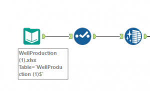
An Excel file is brought into Alteryx using the data import tool, then a Select tool is added to determine the correct data types of the file. Next, a Data Cleanse tool is used to remove any nulls and prepare the data for the next steps.
Creation of Running Total and Start Dates
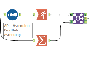
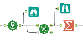
The prepared data now takes two paths before eventually being joined back together using a join tool. The first path (top) sorts the data by API number and production date, then uses a Running-Total tool to create a new column, tracking the well output over time. The second path (bottom) uses a Summarize tool to find the minimum production date for each well. The data is then rejoined.
Filtering for Date Range and Creating Cumulative Totals
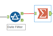
The next step involves filtering the current set of data to only contain records within 6 months of the well start date. This displays the built-in functions of Alteryx. The data is then put through a Summarization tool again to pull the maximum value, thereby providing us with the 6-month cumulative amounts.
Joining of Well Location Data
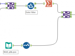
Next, the file containing the well information is introduced to the workflow. This is joined to the existing workflow by the well API number. This allows the demonstration of multiple data types being used together.
Addition of Geo-Spatial Tools
The newly joined latitude and longitude information will be used to create a map. The first tool used is a Create Points tool, which grabs the coordinates and plots them relative to one another. The next tool, Find Nearest tool, allows the points to be related to the nearest four wells within a kilometer. This data will now contain individual data and universal data that can again be summarized.
Categorize the Results, Create a Production Delta, and Output Results
The next step uses another formula to bin the results into a well type category (infill or parent), based on the start data versus the universal start date. The Formula tool is also used to create a field that calculates the difference between a well’s values and the universal values. At this point, the data can be summarized again to see the difference of average performance between infill and parent wells. The data can also be output at this time to just about any file format, and distributed via your preferred reporting and Business Intelligence platform.
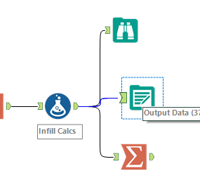
At this point, the output data was shown as a visualization that captivates the audience.
The next examples are focused on the predictive analytics capabilities of Alteryx. The active report tabs were also demonstrated live.
Linear Regression
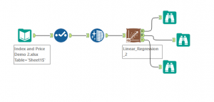
This example used an Excel sheet of actual prices and a series of four indices. The Linear Regression tool is used to show how well each index did in predicting the actual price. The Report and Interactive tabs were explored.
K-Means Clustering
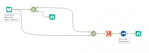
This example used a series of contracts with flags determining their attributes. The tool was used to create clusters of contracts by similar attributes, as well as ranking these clusters by profitability.
Questions? Email us at info@capitalizeconsulting.com for more information!